Assembly
What is Assembly?
Assembly is simply the process of building contigs (longer sequences) from your raw read data. This is generally accomplished now with a de bruijn graph. I would like to make a distinction in terminology here as well. In using software and listening to other talk you may hear the term scaffold. Though some people may use contig and scaffold interchangeably, they are NOT the same thing. A scaffold consists of contigs and gaps, in other words it is an ordered series of contigs with a determined order. This is just something to be aware of.
De Bruijn Graphs
This will be a basic introduction to De Bruijn Graphs. It will cover how the graphs work with one genome and then how this can be applied to a metagenome.
First a note on k-mer lengths. These graphs rely on k-mers to assembly contigs. That being said you can choose any length of k you want in theory. Many have presets that assemble on a range of k-mer lengths. There is one rule to the length of K though. This rule is that the length of K MUST BE ODD. This idea comes from the fact that an even k-mer can end up being the reverse compliment of itself or is palindromic. These sequences make the resolution of the graph difficult and by picking and odd value for k you can eliminate the occurrence completely.
There are four major steps to assembly with De Bruijn graphs:
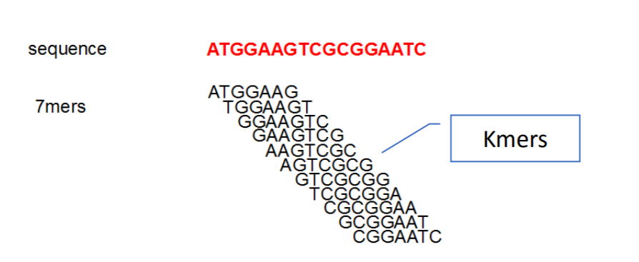
1. Determine k-mers of each read
First each read is broken down into its consecutive kmers
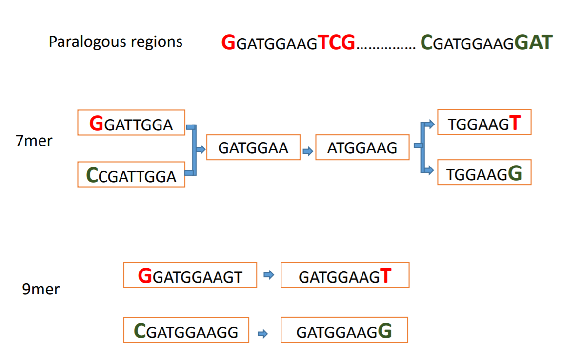
Typically this is done over a range of k-mer lengths because it can help resolve parts of the genomes for example in the following image using a kmer length of 7 creates an ambiguous section of the graph from two sections of the genome while using a 9-mer resolves the section into its two separate parts.
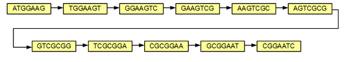
2. Construct the Graphs
Once the kmers are determined they can be arranged in a graph where nodes(holds kmers) are connected if the kmers in the nodes have an overlap of k-1 with each other. in a simple graph where each k-mer only appears in a genome exactly once, like in the first image of the previous sections, the graph would look something like this:
The above graph is extremely simple. An actual graph is extremely complex even for a single species. For example, the following is a graph for the genome of e. coli:
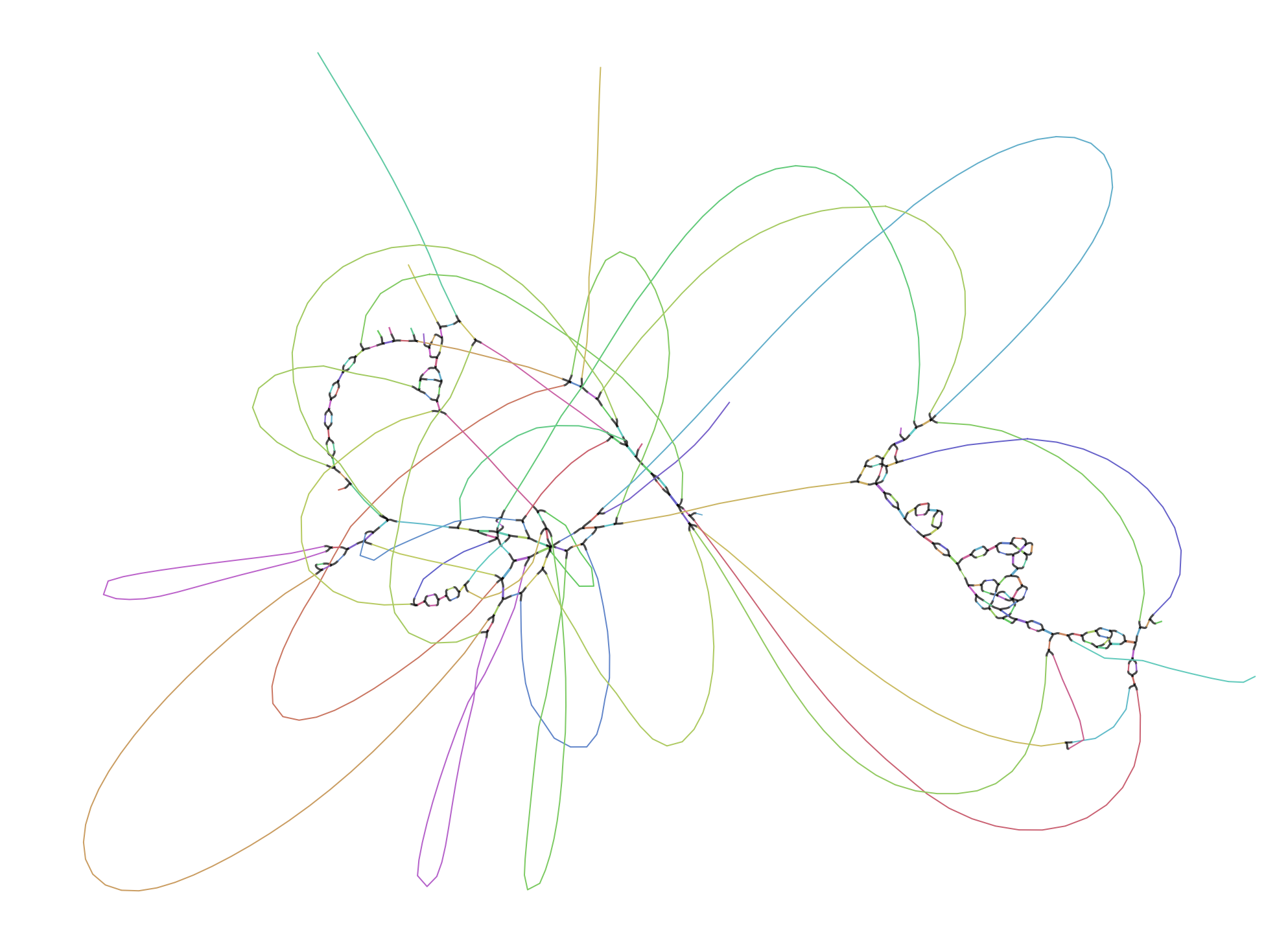
As you can see, it it much more complex and there are major loops and bubbles and other separate pieces from this assembly
3. Graph Simplification
As shown previously, these graphs can become very complex very quickly. Some of this complexity comes from biological reasons while other come from sequencing errors. This section explains some of the complexities that appear and how they are dealt with to get a cleaner more accurate assembly. You may have encountered some of these terms in meetings or readings.
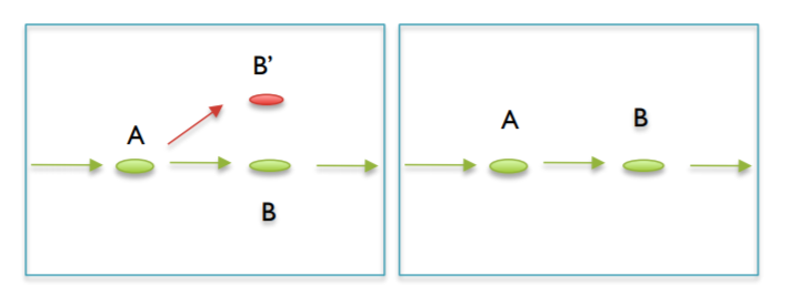
A. Trim Tips
Tips are protrusions from the graph that end in a dead-end. In other words, these protrusions do not loop back in. Tips appear when there are errors towards the ends of the reads. These are simply simply removed. Typically they are removed according to a length threshold and the tip will be kept if it is longer than the threshold.
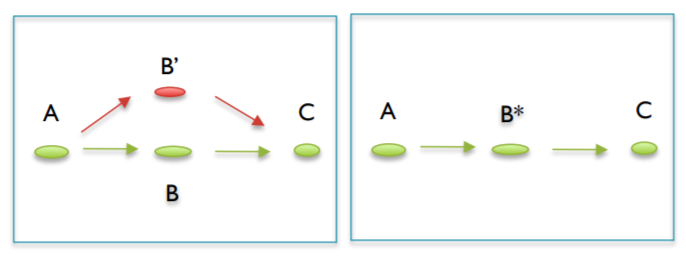
B. Pop/Merge bubbles
Bubbles are areas where a graph deviates by comes back after a short length. Bubbles can appear for many reasons. They can appear from a random overlap of two tips(typically seen in high coverage data sets), an error in the middle of a read, or due to polymorphisms of the genome. Popping/Merging bubbles can occur in many ways, and it uses many metrics such as coverage to decide the correct path or merge the junction.
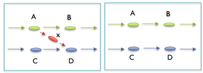
C. Clip Short Low Coverage nodes
This is mainly done to remove chimeric links. These chimeric links are not bubbles or tips, and they connect to longer genuine contigs to each other in ways they they should not be connected. They can be the overlap of two tips, an incorrect read match to an area of the genome it does not belong in, or an actual sequenced chimeric read. These are simply removed.
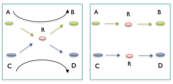
D. Correcting Ambiguous Paths (branches)
some places appear where contigs may share a short section of sequence but aside from that they are independent of each other. Imagine an X where the intersection is the overlapping sequence. These are split into two independent contigs and each of them get the overlapping sequence.
4. Find a Path Through the Graph
Once the graph is cleaned up you can find a path through all the notes to create the contigs. There are multiple solutions to finding the path.
5. Application to a metagenome
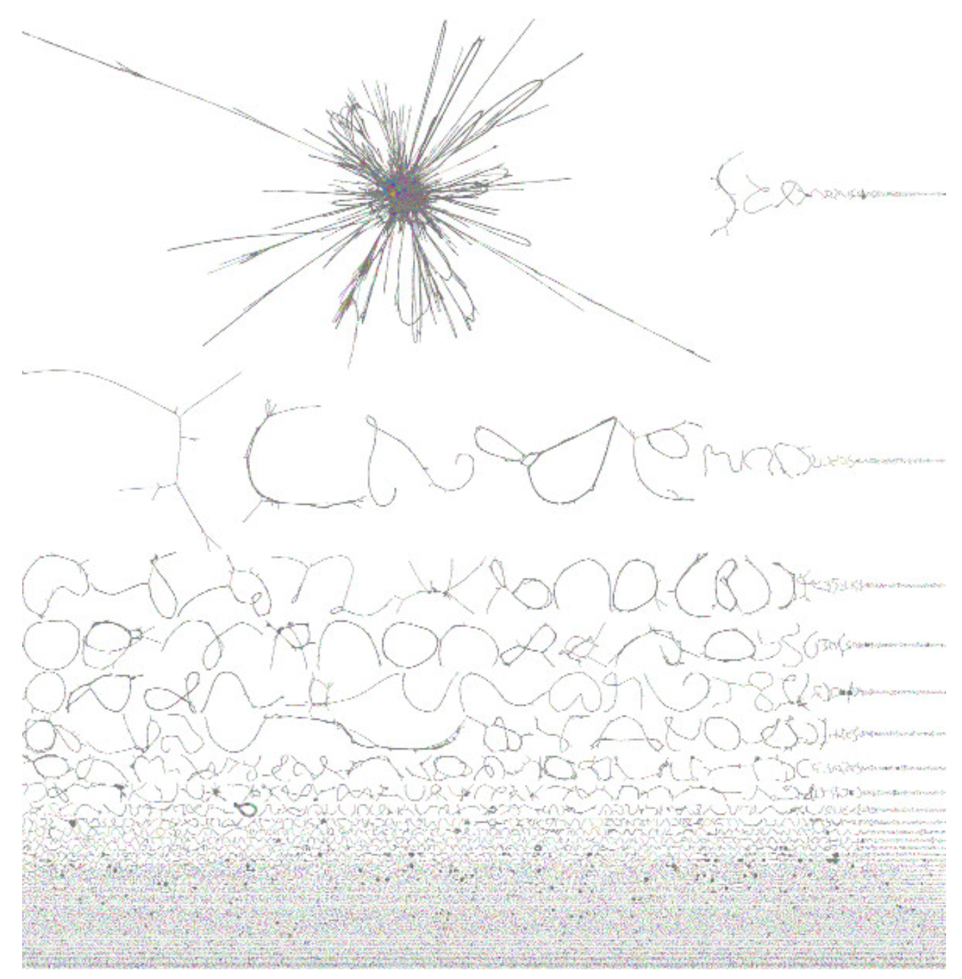
All of the same concepts as above apply. However the graph will essentially section itself off into different genomes. Highly divergent species will appear to separate while highly similar ones will become intertwined with each other. An example visualization of a metagenome can be seen below:
Assembly Considerations
1. Co-assembly
- Benefits of co-assembly:
- higher read depth
- allows comparisons across samples with one reference assembly
- can make binning with differential coverage more powerful
- can bridge contigs to result in a better assembly
- create more consistent contigs
while above are some benefits it is important to note that metagenomic samples can be very fickle and while these benefits may work in some samples, they could not in others.
2. Digital normalization?
Running the software
We use megahit for assembly with the preset range of kmers for sensitive assembly.
For megahit you need your qced fastq files and can run it like this for a single samples where are r1 and r2 are the read1 and read2 files. -t is the number of cores and -o is the output directory.
megahit -1 r1.fastq -2 r2.fastq -t 40 --presets meta-sensitive -o Megahit_meta-sensitive_out/
The command for a co-assembly is the same except r1.fastq and r2.fastq can be replaces with a list of r1s and a list of r2. An automated version of that might look something like this:
# make comma separated lists of fastqs

r1=`ls ../reads/*R1* | python -c 'import sys; print ",".join([x.strip() for x in sys.stdin.readlines()])'`
r2=`ls ../reads/*R2* | python -c 'import sys; print ",".join([x.strip() for x in sys.stdin.readlines()])'`

# run megahit co-assembly
megahit -1 $r1 -2 $r2 -t 40 --presets meta-sensitive -o Megahit_meta-sensitive_out/